Tuning Transitions
The following methods provide mechanisms of updating and generating attune.Instrument objects from measured data in the WrightTools Data format.
This documentation assumes a working knowledge of the WrightTools Data format.
There are four generic methods for working up measurements which each serve to optimize for particular use case. Each section will provide general usage tips as well as provide specific examples of workflows which use the function.
Because all of these methods have many available parameters, all parameters must be specified as keywords, even the required parameters. There are several parameters which are common to all or most of these methods. To avoid repetition, the common parameters are:
- data (all)
An input WrightTools Data object, properly formatted for the routine.
- channel (all, though for holistic it is channels, plural)
The channel from the data object to use as inputs to the workup routine.
- arrangement (all)
The name of the arrangement in the
Instrument.- tune (intensity, setpoint, and plural
tunesfor holistic) The name of the tune in the arrangement specified to update.
- instrument (all, optional for intensity and setpoint)
The
Instrumentto update incorporating the data, if not given a new instrument is created.- level (optional for intensity, holistic, and tune_test)
If
TruethenWrightTools.data.Data.level()is called prior to interpreting the data from the selected channel- gtol (optional for intensity, holistic, and tune_test)
The “Global Tolerance” to ignore data below a multiplicative threshold of the maximum value in the dataset. This is used to cut out noise from the baseline of the data which may pull the selected centers away from their true value.
- ltol (optional for intensity, tune_test)
The “Local Tolerance” to ignore data below a multiplicative threshold of the maximum value in a particular slice. This is used to cut out side peaks or other artifacts that are above the global noise floor, but smaller than the desired peak to fit.
- autosave (optional for all)
This is a boolean of whether or not to save the output instrument and graphical representation into a folder or only keep in memory.
- save_directory (optional for all)
Specifies the location to save the instrument and graphical representation to
The methods all work by generating some spline of best fit through the space that it is optimizing, using the information from the data.
As such, each of the methods also take additional keyword arguments which are passed into the scipy.interpolate.UnivariateSpline.
This can be useful to fine tune the smoothness of the output to ensure desired outcome.
One common use is to forgo smoothing all together by passing s=0, k=1, which makes the spline equivalent to a 1-D interpolator through each chosen point.
tune_test
A tune test allows for quick and easy evaluation that a given arrangement produces good quality light that is true to the color it says it is.
The scan for a tune test is the tune points of the arrangement vs a spectral (monochromator or array detector) axis, which is transformed to be the difference between the actual color and the expected color.
When the system is well tuned, the tune test will be flat at 0 along the differential axis and have adequate power over the expected usable range of the arrangement.
When the system is not well tuned, there will be deviations from 0 along the differential axis. If the tune test is significantly off, or if the intensity is diminished in the expected usable domain, then it is advisable to address the problem using other tuning strategies.
In general, systems which use a setpoint() or holistic() as one of the steps of the tuning procedure will generally not want to apply tune tests results, instead using it only as a diagnostic tool.
This mostly applies to shorter pulse duration OPAs which have less separable motor space and wider bandwidth light, in the femtosecond regime.
OPAs with longer pulse durations often can get by with simpler optimization routines using only intensity() to achieve adequate power over the usable tuning range, but intensity() does not provide any spectral information so tune_test() is used to ascertain the actual output color correctly.
tune_test() generates an updated curve by first identifying the actual color that each tune point produces, using a spline to smoothly interpolate them, then interpolating each tune of the arrangement back onto the original tune points.
tune_test() accepts one additional parameter restore_setpoints which prevents the tune points from being interpolated back if it is set to False.
data.transform("w3", "wm-w3")
out = attune.tune_test(
    data=data,
    channel="signal_mean",
    arrangement="sfs",
    instrument=instr,
)
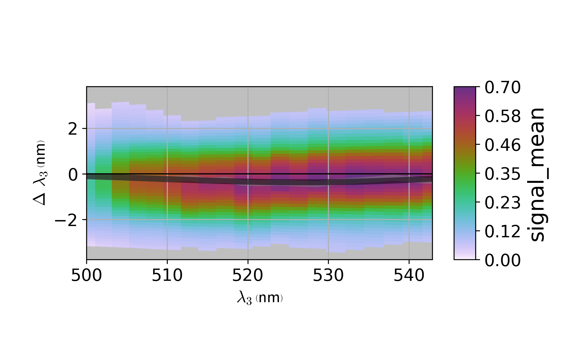
The optimal tune test plot is flat at 0 deviation from expected color.
intensity
intensity() provides a mechanism to update a single Tune in an instrument by optimizing the tune to provide the most intense position at each tune point.
When passing an Instrument to intensity(), it is treated as updating the existing position by adding to the existing positions.
This is the process when updating an OPA motor, which has been scanned as a differential from the previous expected position against the opa tune points.
Any tunes other than the one specified as a parameter are ignored and kept the same as the input Instrument.
This method of tuning is usually sufficient for OPAs in the picosecond regime, where pulse widths allow each motor to be tuned independently.
It is also used for later motors in femtosecond tuning procedures such as the delay_2 motor of a Light Conversion TOPAS-C OPA or any additional mixing process after signal and idler have been generated.
data.transform("w1=wm", "w1_Delay_2_points")
new = attune.intensity(
     data=data,
     channel=-1,
     arrangement="sig",
     tune="d2",
     instrument=old,
 )
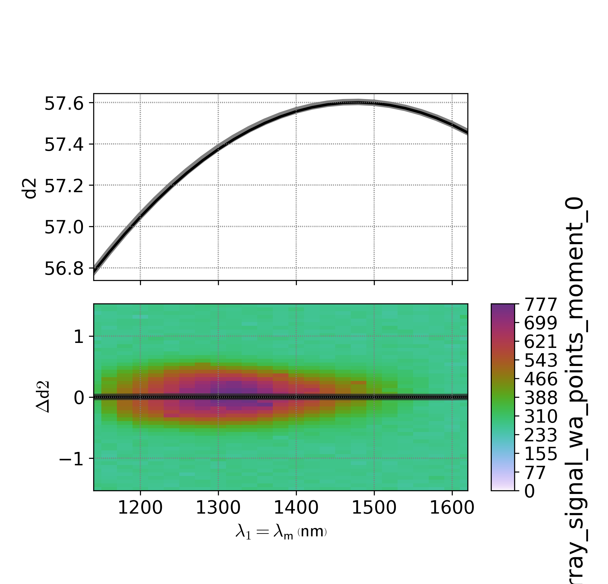
In the plot, the optimal position of the motor would be to follow the ridge of the most intense peak.
When no Instrument is provided, intensity() creates a new Instrument containing only the one tune.
This is the process for generating a Spectral Delay Correction attune.Instrument object.
The scan for SDC is a delay position (usually centered around 0) versus the OPA tune points.
Since the output instrument contains only a single arrangement with a single tune, update_merge() is often used to recombine the SDC output into an instrument which contains SDC tunes for alternate OPAs and arrangements of the same OPA.
setpoint
Instead of optimizing for output intensity, setpoint() optimizes for the correctness of the expected output color.
This is useful for motors in femtosecond OPAs which when perturbed change the overall intensity little, but strongly affect the color produced, such as the Light Conversion TOPAS-C crystal_2 motor.
The scan is nearly identical to the scan required for intensity(), however since it is optimising color information, a spectral axis (either via scanning a monochromator or via an array detector) must be used.
The data must be transformed to (setpoint, differential_motor_position)
The channel must be pre-processed to contain the color information, rather than intensity information.
This is usually done by taking the WrightTools.data.Data.moment() with moment=1 along the spectral axis of the scan.
data.transform("w1=wm", "w1_Crystal_2_points", "wa-w1")
data.level(0, 2, 5)
data.array_signal.clip(min=0)
data.transform("w1=wm", "w1_Crystal_2_points", "wa")
data.moment("wa", moment=1, resultant=wt.kit.joint_shape(data.w1, data.w1_Crystal_2))
data.transform("w1=wm", "w1_Crystal_2_points")
data.channels[-1].clip(min=data.w1.min() - 1000, max=data.w1.max() + 1000)
data.channels[-1].null = data.wa.min()

out = attune.setpoint(
    data=data,
    channel=-1,
    arrangement="sig",
    tune="c2",
    instrument=instr,
)
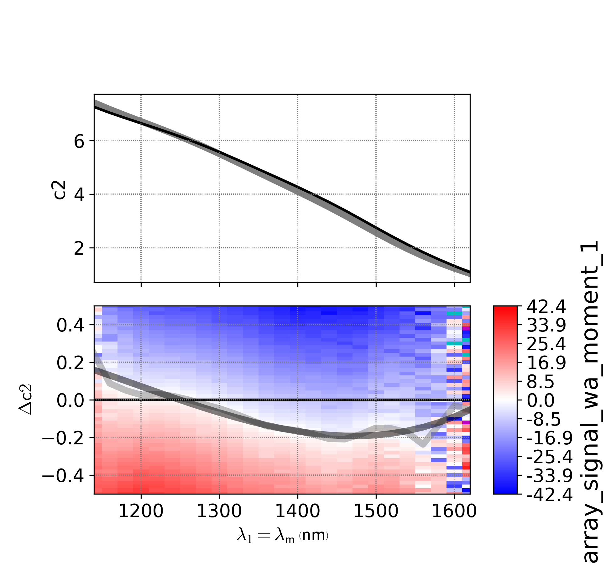
In the graph, the color represents deviation from the expected color and pure white is the optimal motor position.
holistic
holistic() takes a multidimensional approach by using both intensity and color information to optimize two motors at once.
This is most useful for femtosecond OPAs where some motors are not separable due to bandwidth of the pulse.
As such for the Light Conversion TOPAS-C OPAs, this is used to tune the “preamp” or crystal_1 and delay_1.
The scan for holistic actually looks very similar to the scan for setpoint, including the OPA setpoint axis, a differential motor axis, and a spectral axis (which could be from an array detector). However, instead of being transformed to include the OPA setpoints, the transform is applied such that two motors are in the transform.
holistic() can either be handed separate intensity and spectral channels (as a 2-tuple channels argument) if separate preprocessing outside of the scope of the method is required.
In this case, it expects each channel to be two dimensional and no spectral axis to be present in the channels or transform of the data.
If it is given a single channel it expects that the spectral axis to be present and will take the 0th and 1st WrightTools.data.Data.moment() to get intensity and spectral information, respectively)
The spectral axis is assumed to be the last axis of the transform as provide, but can be overridden using the spectral_axes parameter.
The algorithm for holistic() starts by clipping data below the gtol for the amplitude channel, applying the clip to both the amplitude and color channels (as you cannot get a reliable color estimate from values below the noise threshold).
It then creates a scipy.interpolate.LinearNDInterpolator for each of the amplitude and spectral channels.
It finds the point on each edge of the scipy.spatial.Delaunay interpolation triangles which are the color of each tune point.
If enough points are found that are the requested color, it fits the points to a Gaussian function using the intensity information, one Gaussian for each dimension.
It then splines each motor against the input color, and replaces the tunes in the input instrument with the new splined positions.
In principle, this algorithm generalizes to an arbitrary number of dimensions, however the plotting step in particular only works for 2 dimensional data.
data.transform("w1_Crystal_1", "w1_Delay_1", "wa")
out = attune.holistic(
    data=data,
    channels="array_signal",
    arrangement="NON-NON-NON-Sig",
    tunes=["c1", "d1"],
    instrument=instr,
    gtol=0.05,
    level=True,
)
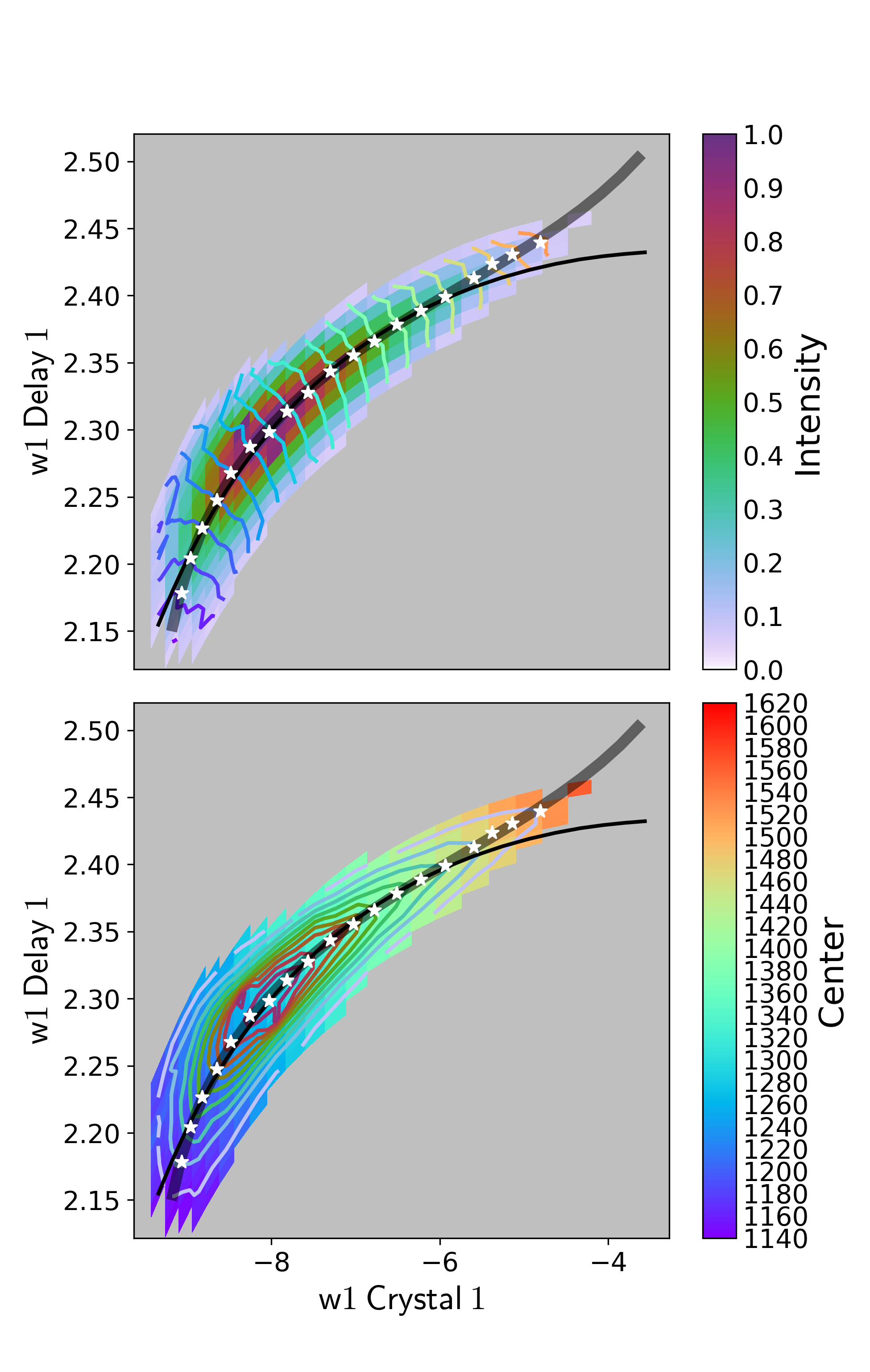
The axes of both plots are in 2D motor-space. The top plot is an intensity plot with contours of constant color overlaid. The bottom plot is the inverse: color plot with contours of constant intensity overlaid. The thin black line is the input path through 2D motor space. The thick semitransparent line is the output selected path through 2D motor space. The stars are the points which were selected by the algorithm for each tune point. Ideally, the thick black line would be along the ridge of the “slug” shape.